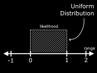
Imagine closing your eyes and placing your finger somewhere in the shaded region in this image. Notice that at any point in the range from 0 to 1, there is an equal likelihood that your finger will be above a given point. There is NO chance you will place your finger outside the range, you are skilled with your eyes closed!
Now conveniently, we can use math to modify the value that we place our finger above. Say we multiply whatever value we receive by 2. How have we affected the result? Well put simply, we have increased the range of our value. Now instead of being between 0 and 1, the value will be between 0 and 2. But we retain the property that any value in this range is equally likely.
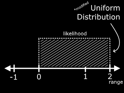
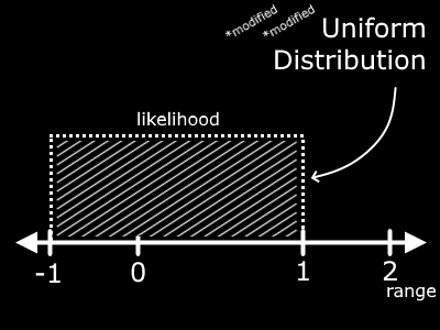
Cool! So that makes sense. You can twist and turn this range all you want by adding, subtracting, etc. For example, if we subtract 1 from this new range, we manage to shift it down by, you guessed it, 1.
Straightforward, right? If you are an experienced programmer or you know math well, this may seem trivial to you. But now I'll provide some more interesting insight.
No matter what we do - add, subtract, multiply, divide by constants - we will always retain this property of equal (or better yet, uniform) likelihood. But there are ways that we can change this property to some other, what is called, distribution.
A simple example is if we take the first value from the range of 0 to 1 and multiply it by itself. You may know this as... not triangling or circling... but squaring the value. This will cause an important change in the graph.
Well would you look at that! We no longer have the flat line representing the likelihood. Now, it is a curve. If you examine the graph, you should be able to work out in your mind that small values in the range 0 to 1 are more likely to find our falling finger. The area near the right end (at 1) is much smaller than the area around 0.
Now, you should be wondering why exactly value are more likely to be near 0 than 1. Time for some math - but don't worry, it is simple math! What is the value of 0, squared (I'll use this notation: 02)? Well multiplying 0 x 0 results in a value of ... well 0! What about 12? 1 x 1 = 1. This math is super simple. Now for a more interesting multiplication. What is (0.5)2? Well if you plugged this in your calculator, you would find a value of 0.25. What about 0.92? What about 0.12? I'll write down some common values below.
02 = 0
0.12 = 0.01
0.22 = 0.04
0.52 = 0.25
0.92 = 0.81
12 = 1
The moral of the story is, when you square a value between 0 and 1, it becomes smaller. With this logic, it is more likely that the value is small than large. I have made it a point to emphasize what is going on here because, well, it is important to understand how we will be working with the uniform distribution.
Now, time for something cool. Remember the "*modified *modified Uniform Distribution" from above? Well recall that it was a uniform distrubtion taking values between -1 and 1. Consider any value in that range, squared. We just figured out what the graph will look like between 0 and 1. If you know anything about negative numbers, it should at least be that a negative times a negative becomes a positive.
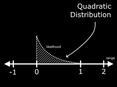
With a little intuition, you may reason that the final distribution should look something like this:
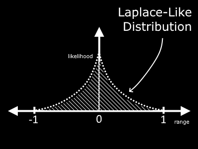
This shows that by taking the original uniform distribution in the range -1 to 1 and squaring it, we are much more likely to find values closer to 0 than we are near 1 or -1.
This looks like a Laplace Distribution. The name of this isn't so important, and truth be told it is not even the correct equation to find this particular distribution (I call it Laplace-like), but the point is that we have emulated a certain probability distribution with a simple translation from a uniform distribution. How fascinating!
We could take it upon ourselves to modify this even more! Say we want a range of -4 to 4. Multiplying by 4 would suffice! We could even square the value again to get a tighter slope around 0, which makes values near 0 very likely. The world is your playground!
Now, for the final part of this blog post: the Normal Distribution. The normal, or Gaussian, distribution is a very common distribution that we observe in the real world. What I want to cover here is how to convert from a uniform distribution to a normal distribution.
The simplest way I have found to emulate a normal distribution is with the tangent function. The plot of tangent is shown below.
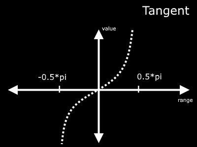
The range of the input to tangent should be between (-0.5*pi) and (0.5*pi). Using methods towards the beginning of this post, we can change our range to match this quite easily. First, subtract 0.5 to change the range to -0.5 to 0.5. Then simply multiply by pi!
uniform = rand();
mod_uniform = (uniform - 0.5) * pi;
Consider now that the value we found within the new range of tangent is going to be used as the input to the tangent function. What output value from tangent should we expect? Well most of the time, the value will be near 0. Only rarely (when the input is near an extreme) will the value stray significantly away from 0. And to add another new phenomena, the output range has been extended to infinity. Woah.
normal = Tangent(mod_uniform);
If you run many samples through this random generator and plot them, you will find an output that resembles this curve (the Bell Curve).
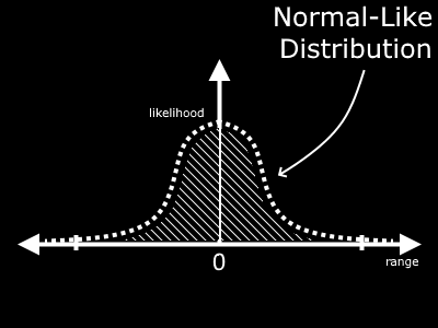
Values near zero are extremely likely, but there is a small chance of values outside the typical range of -1 to 1 or even -0.5*pi to 0.5*pi. You could even find a value of 100 every once in a great long while, but it is extremely unlikely.
So, we have arrived! The normal distribution appears all over the place in the real world, especially where probability and random processes are concerned. One example I can think of is, say you are programming a tree generation system. Well, it turns out that most trees grow to be a certain height, but there are occasional odd-balls. Maybe you want some trees to grow shorter and some to grow taller, but rarely. Well guess what, the normal distribution may be exactly what you are looking for!
Many programming languages include the capability to pull directly from a normal distribution. randn exists in python and MATLAB. But some popular languages do not have this option. Javascript and C/C++ are examples. By implementing a simple funciton with Tangent, you can achieve your desired result.
If you would like to see this in action, I threw together a quick demonstration using the method I discussed in this article found at this link.
A brief disclaimer: this distribution is NOT precisly normal. It does not have the correct value of standard deviation. If you are looking for a more precise distribution, check out the Box-Muller Transform. It is similar, but with more precise control. It does require more computation though.
I hope you learned something! Random number generation is a very interesting topic, we are only scratching the surface.
Be Curious!